3.3 Genetic drift

Consider the following simplified model of evolution of a single position of the genome: we have a starting population of \(N\) people (and so, \(2N\) copies of the genome since we are diploid). The position has two alleles, A and B, with frequencies p and 1-p in the population. We will assume that the population size is constant at \(N\) people over time, and that generations are non-overlapping. So, every generation, we have \(N\) new individuals. Their two alleles are each drawn at random from the \(2N\) available alleles from the previous generation. This process happens over and over again over many generations of evolution.

This simple process of genetic drift is formalized in the Wright-Fisher model. If there are \(2N\) total alleles, and the frequency of A is \(p\), then the probability that there will be \(k\) copies of A in the next generation can be computed using the binomial distribution:

\[P(k \text{ copies of } A) = {2N \choose k}p^k(1-p)^{2N-k}\]

This process gets repeated each generation. Note, each generation we must recompute \(p\) based on the observed frequency of A in the previous generation.

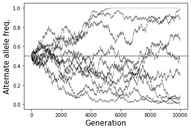
The figure below illustrates the process fo genetic drift in simulated data. Each line shows a different random simulation. The x-axis is the number of generations that have passed, and the y-axis is the frequency \(p\) over time, which started at \(p=0.5\):

The Wright-Fisher model is essentially a simple random walk. Note that both \(p=0\) and \(p=1\) are absorbing states. In the absence of new mutations, once we reach an absorbing state, we are stuck there forever. i.e. once either A or B disappears, the allele frequencies will stay constant in all future generations. We call this fixation of one of the alleles (and loss of the other). If we run the evolution process for enough generations, eventually we will reach one of these absorbing states.

Some interesting properties about patterns of genetic variation in populations can be derived from this model:

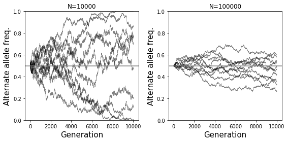
• Effects of population size: The smaller the population size, the more dramatic effect genetic drift will have. If a population is very large, frequencies will remain pretty stable across generations due to the law of large numbers. In the extreme case of infinite population size, allele frequencies will stay constant. On the other hand, if a population is very small, due to sampling noise there may be large fluctations in allele frequencies each generation. The simulations below show how the behavior of drift is different in small (left) vs. large (right) populations.

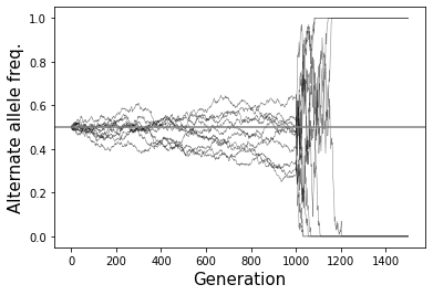
• Effects of population bottlenecks: A population bottleneck occurs when a small group of founder individuals from an original population forms a new population group, creaing a substantial reduction in population size. This can have dramatic effects on allele frequencies. For example, if an allele that was originally rare was present in one of the small number of founrders, that allele may suddenly become common in the new bottlenecked population. One consequence is that populations such as Ashkenazi Jews, early French Canadian settlers, and Finnish, which experienced recent bottlenecks, have a high rate of recessive disorders which are rare in other groups but common in the bottlenecked groups since they happened to be carried by some of the original founders. The simulations in the figure below were generated with a population size that starts at 10,000 then drops to 50 at generation 500. You can see nearly all alleles quickly go to either fixation or loss.

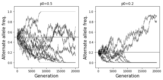
• Effects of allele frequencies: An allele that is at 50% frequency as a 50% chance to eventually be lost or become fixed. An allele that is rare is more likely to eventually be lost. On the other hand, an allele that is very common is likely to eventually take over and become fixed. Formally, the probability that an allele with frequency \(p\) will eventually be fixed is equal to \(p\). The time it takes for fixation to occur is proportional to the population size. Fixation will happen more quickly in small populations and take a long time in large populations.

The simulations below show how the behavior of drift is different for an allele with starting frequency of 0.5 (left) vs. 0.2 (right). In the second case, loss is more likely and happens more quickly than when the starting frequency is 0.5.