7.4 GWAS for case-control traits

In previous sections we focused on GWAS for quantitative traits. In some cases, we will instead have case-control traits, in which our phenotype is a binary outcome (e.g. 0=control, 1=case) instead of a quantitative value. In this case, the linear regression technique we used previously is not the most appropriate test to use. We’ll discuss two alternatives.

7.4.1 Chi-square test for case-control traits

Let’s consider a single SNP, with alleles T and G. We’d like to test for association between the genotypes at this SNP and a case-control phenotype. We could start by making a table of how many times we saw each genotype (TT, TG, or GG) in either cases or controls:

	TT	TG	GG	total
controls	\(r_0=25\)	\(r_1=50\)	\(r_2=25\)	\(R=100\)
cases	\(s_0=64\)	\(s_1=32\)	\(s_2=4\)	\(S=100\)
total	\(n_0=89\)	\(n_1=82\)	\(n_2=29\)	\(N=200\)

Now, we can convert that to a table of how many times we saw each allele:

	T	G	total
controls	A=\(2*r_0+r_1=100\)	C=\(2*r_2+r_2=100\)	\(2R=200\)
cases	B=\(2*s_0+s_1=160\)	D=\(2*s_2+s_1=40\)	\(2S=200\)
total	\(2n_0+n_1=260\)	\(2n_2+n_1=140\)	\(2N=400\)

Now we’d like to ask: is one allele over-represented in cases vs. controls?

We can compute an odds ratio for a particular allele. Let’s define:

• The odds that T occurs in a case: \(B/A\)

• The odds that G occurs in a control: \(D/C\)

Then the odds ratio for allele T is defined as:

\[ OR(T) = \frac{B/A}{D/C} = \frac{BC}{AD} \]

In this case, we get the OR=4. That is, the odds that a T occurs in a case is 4 times higher than the odds that a G occurs in a case.

We’d also like to get a p-value to assess whether this is statistically significant. In this case, the null hypothesis is that the OR=1. An OR\(>\)1 indicates that allele T increases risk, whereas an OR\(<\)1 indicates that it decreases risk. We can use a Chi-square test to do this. A Chi-square test compares the observed vs. expected counts. We can compute the expected counts in each cell in our table, assuming the alleles were equally distributed in the cases and controls:

	T	G	total
controls	\((2n_0+n_1)(R/N)=130\)	\((2n_2+n_1)(R/N)=70\)	\(2R=200\)
cases	\((2n_0+n_1)(S/N)=130\)	\((2n_2+n_1)(S/N)=70\)	\(2S=200\)
total	\(2n_0+n_1=260\)	\(2n_2+n_1=140\)	\(2N=400\)

For a Chi-quare test, we just take the sum: \(\sum_i \frac{(obs_i-exp_i)^2}{exp_i}\) which should follow a \(\chi^2(1)\) distribution. We can use the resulting statistic compute a p-value. For our example:

\[ \sum_i \frac{(obs_i-exp_i)^2}{exp_i} = (100-130)^2/130 + (160-130)^2/130 + (100-70)^2/70 + (40-70)^2/70 = 39.6 \]

We can use the CDF of a Chi-square distribution to convert this to get a p-value:

from scipy import stats
1 - stats.chi2.cdf(39.6, 1) # result: 3.18e-10

We get a highly significant p-value, meaning we reject the null that the OR=1.

Let’s check our answer with Python’s chi-square test in scipy:

stats.chi2_contingency([[100,160],[100,40]], correction=False)
# (39.56043956043956, 3.180615853514648e-10, 1, array([[130., 130.],
       [ 70.,  70.]]))

Our answer aggrees with scipy! (the first two values are the chi2 statistic and p-value).

In practice, you can use plink to perform GWAS for case-control phenotypes using a chi-square test with the plink --assoc option.

7.4.2 Logistic regression for case-control traits

An alternative to the chi-square test is to perform a logistic regression. Whereas linear regression was appropriate for fitting quantitative trait values, logistic regression is more suitable for fitting values that are with 0 or 1:

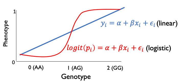
(Note, the logistic line above isn’t drawn quite right… it should plateau at 0 and 1).

The logistic curve can be described as:

\[ p(x) = \frac{1}{1+e^{-\alpha+\beta x}} \]

where \(x\) is a genotype (0, 1, or 2) and \(p(x)\) is the expected phenotype given that genotype. we can rearrange this to write:

\[ logit(p(x)) = \alpha + \beta x \]

where \(logit(p(x)) = \log \frac{p(x)}{1-p(x)}\). That is, the logit function is giving the log of the odds of having a case phenotype if you have genotype x. So we can interpret \(\beta\) as the increase in the log of the odds for each copy of the alternate allele. It follows then that \(e^{\beta}\) gives the estimated odds ratio.

Similar to in linear regression, we can obtain a p-value testing the null hypothesis that \(\beta=0\) (or put a different way, \(e^{\beta}=OR=1\)). (derivation not shown).

Using our example above:

import statsmodels.api as sm 
X = np.array([0]*25+[1]*50+[2]*25 + [0]*64+[1]*32+[2]*4).reshape(-1,1)
X = sm.add_constant(X)
Y = [0]*100 + [1]*100
log_reg = sm.Logit(Y, sm.add_constant(X)).fit()
log_reg.params # for intercept, beta
array([ 0.94000726, -1.38629436])

We estimate an odds ratio of -1.386 (for allele G). This comes out to np.exp(-1.386)=0.25 if we consider G as the risk allele, or 1/0.25=4 if we consider T as the risk allele. Same as above for our Chi-square test!

The major advantage of using a logistic regression vs. a chi-square test is we can add covariates. For example, we might want to control for age, sex, or population PCs. We can simply do so by fitting a model with additional terms, e.g.:

\[ logit(p) = \alpha + \beta x_i + \sum_k \gamma_k PC_{ki} \]

Note, our example had a really large odds ratio compared to what we typically see in GWAS. Typical odds ratios are in the range of \(\sim 0.9-1.1\).

7.4.3 Dealing with case-control imbalance

Logistic regression for GWAS may be problematic if there is a strong imbalance between the number of cases vs. controls or in cases where the minor allele count is very low. In these cases, extensions to logistic regression may be required. See Firth logistic regression and saddle point approximation strategies, both of which are discussed in the REGENIE paper.